Validation and Benchmarks

SymbolicLongMemorySequences.jl separates package correctness from empirical research evidence. Fast tests protect public contracts; validation scripts provide reproducible scientific diagnostics; benchmarks provide machine-specific performance evidence.

See also VALIDATION_POLICY.md, validation/README.md, and benchmark/README.md in the repository.

Fast Tests

Run the package test suite from the repository root:

julia --project=. -e 'using Pkg; Pkg.test()'

These tests are the main development path. They cover deterministic contracts such as constructor validation, output length, element type, alphabet membership, reproducible RNG use, factory discovery, and INC provenance metadata. They also include small seeded statistical checks where exact assertions are not meaningful.

Manual Validation Studies

Manual validation scripts live in validation/. They use reproducible RNGs and may write aggregate result tables or SVG/PDF plots.

julia --project=. validation/marginal_control.jl
julia --project=. validation/local_structure.jl
julia --project=. validation/lrd_method_diagnostics.jl
julia --project=validation validation/longmemory_comparison.jl

Validation scripts may use make_generator for smoke tests of standard cases, but studies that support method-specific claims should prefer explicit constructors so the scientific parameters and assumptions remain visible.

Marginal Control

validation/marginal_control.jl compares empirical frequencies against declared targets across sequence lengths, alphabet sizes, and marginal distributions. It reports aggregate total-variation and maximum absolute marginal errors.

This study is designed to test user-facing marginal controls, not to estimate a Hurst parameter.

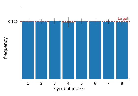
The script also writes a focused uniform categorical validation case for reports and the paper. It uses k = 8, generates n = 100_000 symbols per replicate, drops the first and last 10% of each sequence, and compares the remaining frequencies with the intended uniform marginal. Retained outputs are written under validation/results/marginal_control/:

• uniform_marginal_k8_summary.csv;
• uniform_marginal_k8_histogram_data.csv;
• uniform_marginal_histograms_k8.svg;
• uniform_marginal_histograms_k8.pdf when an SVG-to-PDF converter is available;
• production/marginal/<method>_uniform_marginal_histogram_k8.svg and .pdf for the worst trimmed-total-variation method in the current run.

The summary includes chi-squared frequency diagnostics. Their p-values use the iid multinomial reference distribution and should be read as approximate frequency diagnostics because the generated LRD sequences are dependent. LRD can make empirical marginals converge more slowly than the iid reference assumes, so the strict chi-squared p-values are usually conservative but still indicative. The summary also includes an approximate ESS-adjusted diagnostic. It estimates the integrated autocorrelation time of each centered one-hot symbol indicator, uses the smallest symbol effective sample size as a conservative effective_n, and scales the chi-squared statistic by effective_n / trimmed_n. The adjusted p-values are still diagnostics, not exact dependent multinomial tests, but they are more informative for strongly dependent marginal counts. The summary also includes full-sequence total-variation and maximum absolute errors in addition to the trimmed-window values. That distinction prevents rank-binned or calibrated property-based methods from being misread: they may match the whole generated sample almost exactly while an interior window still wanders because the sequence is dependent.

Better formal tests should calibrate against the dependence structure. Natural extensions are block/subsampling tests or parametric Monte Carlo envelopes generated from the same configured generator. These are manual-validation tools rather than fast package tests.

For MB1a (LAMP) and MB1b (DyadicLAMP), the marginal-control study uses lamp_repeat_transition(p; repeat_probability = 0.4). This is still repeat-biased, but the transition matrix is ergodic with the requested marginal as its stationary distribution. The pure identity transition remains available as a stress case, but it can preserve early finite-sample imbalances for a long time.

Local Structure Control

validation/local_structure.jl measures row-wise and aggregate transition-matrix total variation for WaveletMarkov and OnOffMarkov under validated MarkovSpec values.

The study uses identical MarkovSpec values in each regime when it needs an unambiguous aggregate bigram target. Mixtures of different regimes may be useful generators, but they do not generally have a simple aggregate Markov target.

For large alphabets, a full transition-matrix test needs enough observations in k^2 cells. Shorter one-step diagnostics can test repeat probability, stationary-weighted row total variation, selected rows, grouped symbol transitions, or a few contrast-vector projections of the transition matrix. Those summaries are less complete than a full matrix test, but they need much less data and are often aligned with the intended local behavior.

LRD Method Diagnostics

validation/lrd_method_diagnostics.jl creates one-hot symbol diagnostics for all implemented methods. Property-based methods additionally report diagnostics for the numerical latent process returned by generate_with_latent. Each symbol sequence is transformed into centered indicator series before autocorrelation, autocovariance, or periodogram calculations:

x_t = 1{X_t = symbol} - mean(1{X_t = symbol})

Centering removes the symbol marginal so the summaries focus on dependence rather than zero-frequency mass. Zero-variance indicator series are skipped.

The script writes:

• average_autocorrelation.inc;
• average_power_spectrum.inc;
• latent_average_autocorrelation.inc;
• latent_average_power_spectrum.inc;
• plot_autocorrelation_logbins.inc;
• plot_power_spectrum_logbins.inc;
• latent_plot_autocorrelation_logbins.inc;
• latent_plot_power_spectrum_logbins.inc;
• paired SVG plots under validation/results/lrd_diagnostics/plots/, with autocorrelation on the left and power spectrum on the right;
• title-free production SVG/PDF panels under validation/results/lrd_diagnostics/production/acf/ and validation/results/lrd_diagnostics/production/spectrum/, with ACF and spectral-density plots separated for paper subfigures.

Plot typography or layout can be refreshed from the stored all-method .inc tables without recomputing sequences:

include("validation/lrd_method_diagnostics.jl")
redraw_lrd_diagnostic_plots()

Selected methods can also be recomputed in place without creating separate result folders:

include("validation/lrd_method_diagnostics.jl")
run_lrd_diagnostics(; methods = (:MB4a, :MB4b, :MB4c), write_tables = false)

This keeps plots under validation/results/lrd_diagnostics/plots/, updates the matching production ACF/spectrum panels, and avoids replacing the all-method .inc tables with subset data.

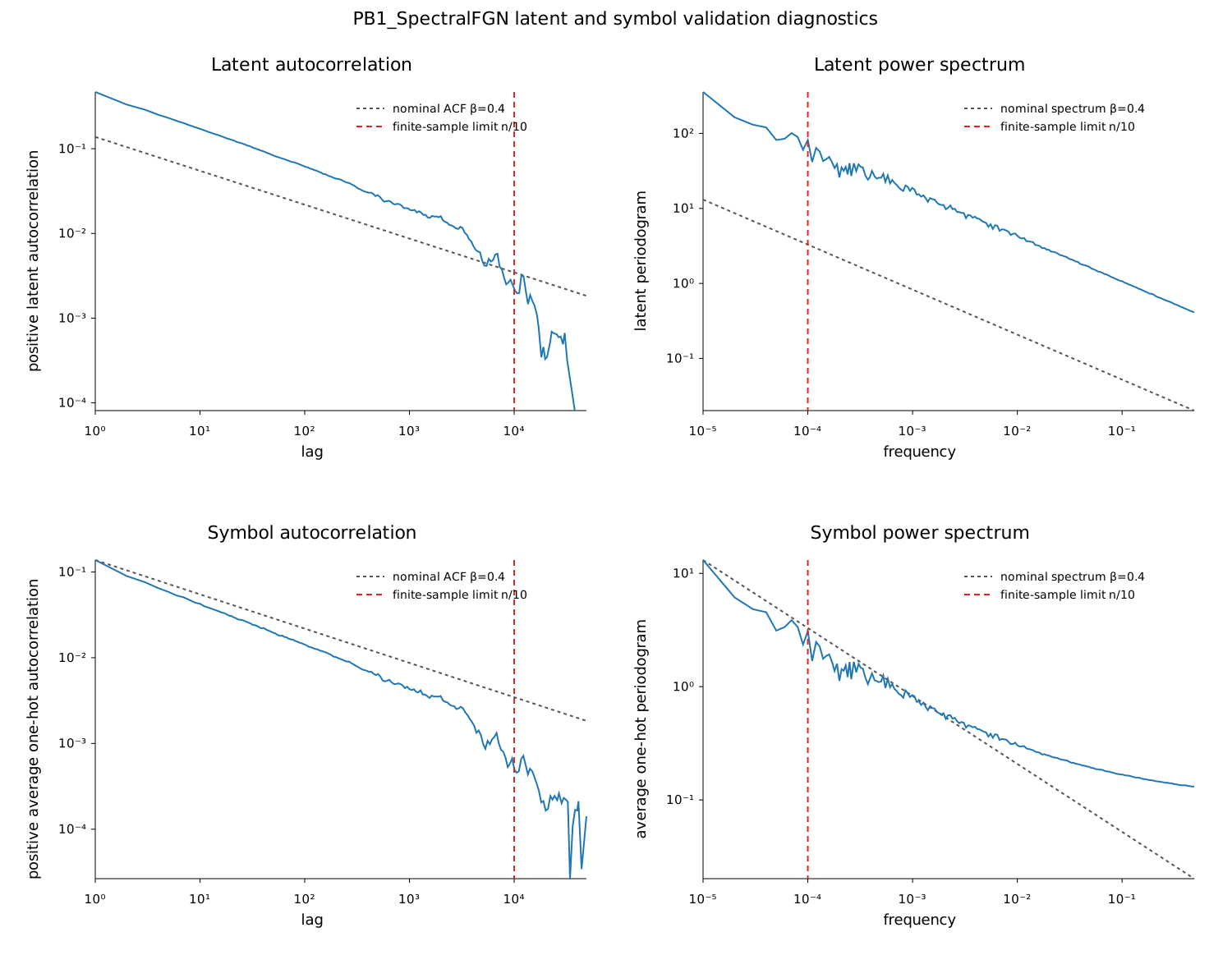
For property-based methods the paired SVG/PDF plots have four panels: latent autocorrelation, latent power spectrum, symbolic autocorrelation, and symbolic power spectrum. The production folder stores the same evidence as separate latent and symbolic panels, making it easier to include only the ACF plots in a paper while retaining the spectral diagnostics as generated artifacts.

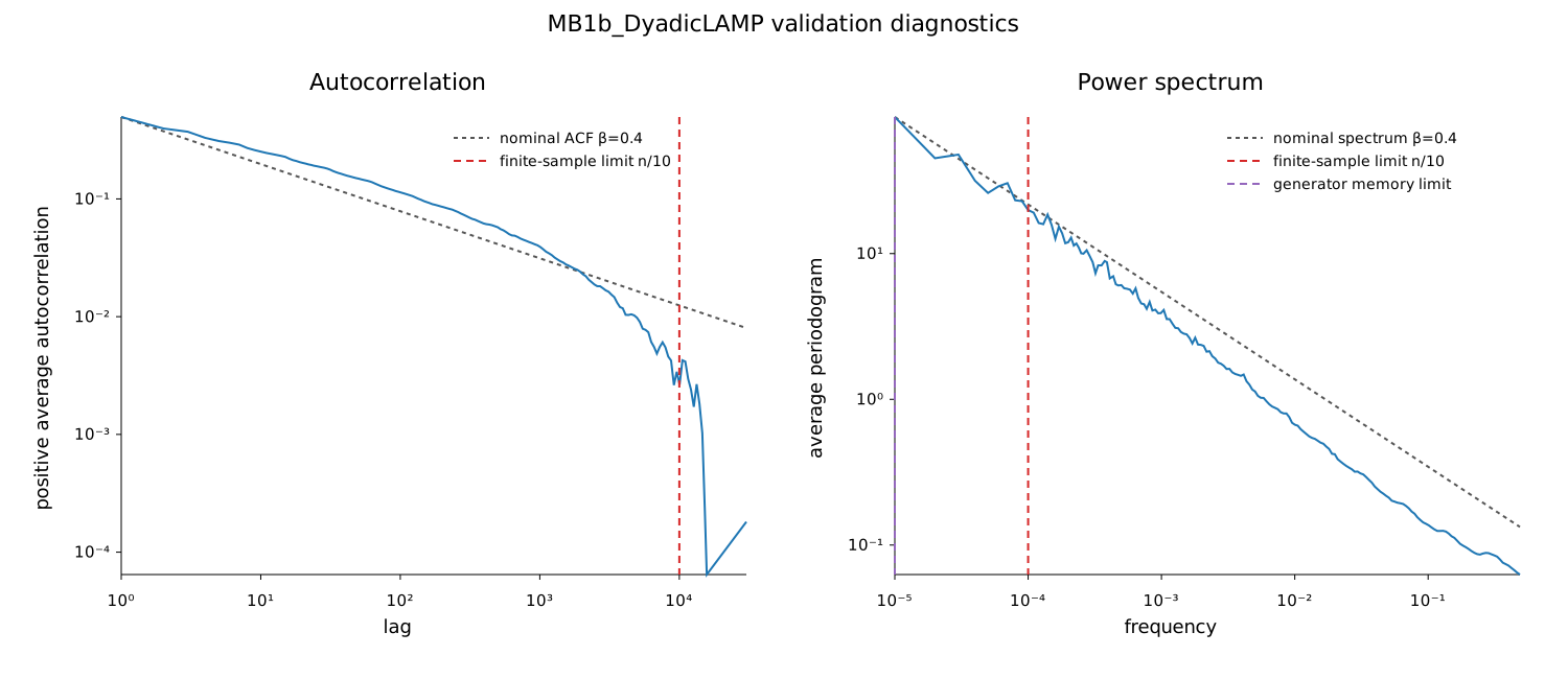
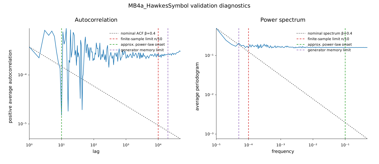
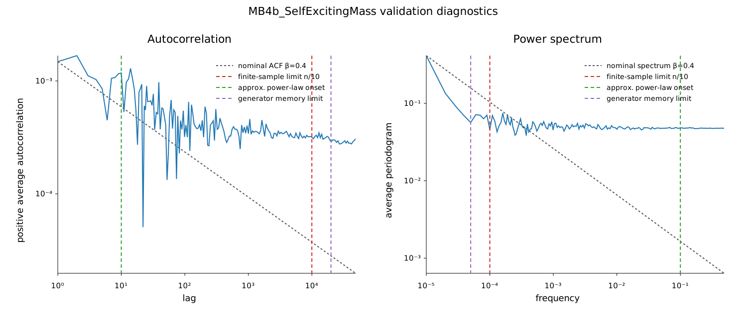
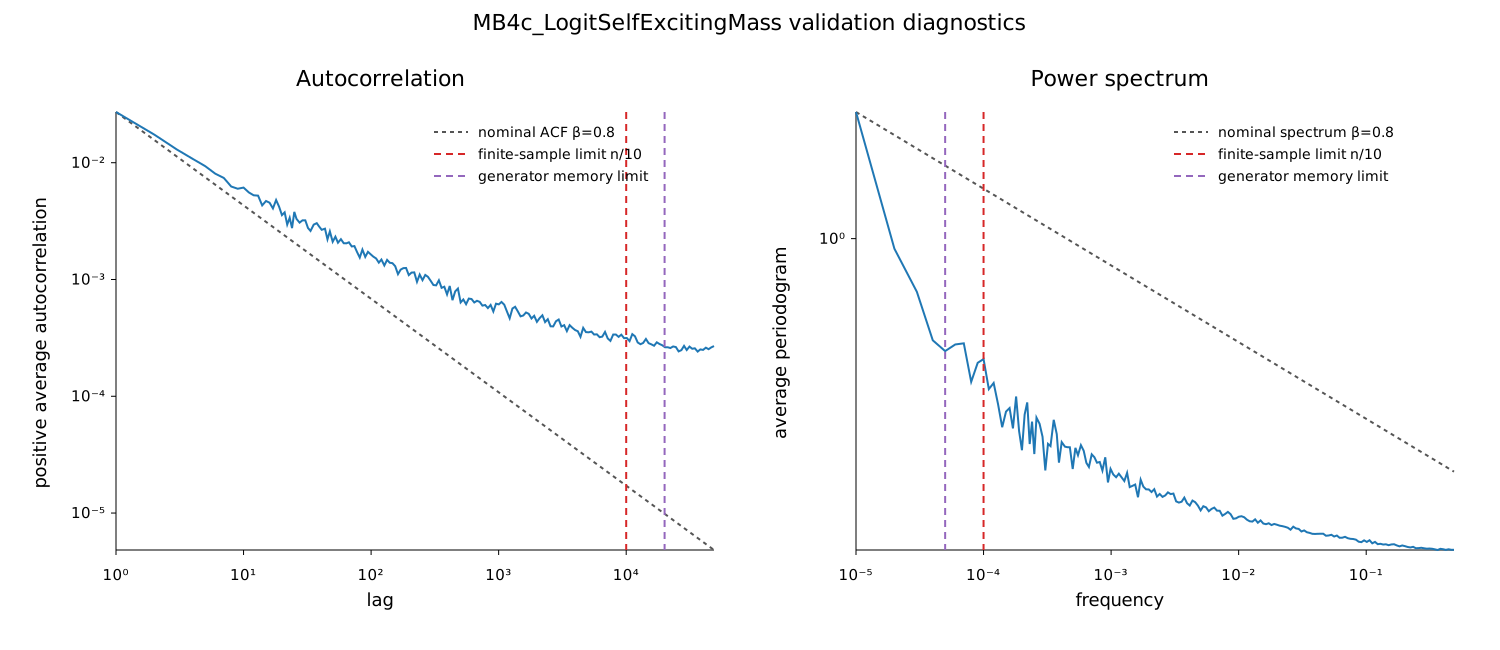
Autocorrelation plots include a vertical dashed finite-sample interpretation limit at lag n / 10. Methods with explicit finite memory, such as LAMP, DyadicLAMP, CalibratedAdditiveMarkov, HawkesSymbol, and DuplicationMutation, also mark the generator cutoff. Power-spectrum plots show the reciprocal scales. Methods with a defensible asymptotic-onset scale also mark an approximate power-law onset: OnOffMarkov uses its Pareto scale L_min, and the MB4 variants use the lag where the local log-log slope of (lag + c)^(-beta) reaches 90% of its asymptotic slope. Gray dashed reference lines show the nominal power-law slope implied by each generator's configured decay parameter; they are visual guides, not fitted curves and not proofs of LRD behavior.

The MB4a (HawkesSymbol) plots are a cautionary case. The finite discrete-time, probability-normalized implementation can produce short-range burstiness while its centered one-hot power spectrum remains close to white noise. MB4b (SelfExcitingMass) leaves the power-law history mass unnormalized until the final categorical probability normalization, with default and smoothing mass retained for support. MB4c (LogitSelfExcitingMass) goes one step further by sampling from centered log-mass contrasts, which reduces common-mode mass normalization. Treat MB4b and MB4c as empirical candidates: MB4c can steepen the spectrum, but too much contrast can lock the process onto too few symbols.

Example Validation Plots

The retained validation run writes plots for every implemented method. The examples below show the main diagnostic styles without reproducing the whole figure set on this page.

PB1 shows the property-based layout. The upper row diagnoses the numerical latent LRD source, while the lower row diagnoses the emitted symbolic sequence after rank quantization.

MB1b is the scalable dyadic-history LAMP variant. Its plot shows the paired symbol-level autocorrelation and spectrum used for model-based methods.

The MB4 variants are deliberately shown together because their validation behavior is part of the package narrative. MB4a is the normalized Hawkes-style baseline; MB4b keeps unnormalized self-excitation mass until the categorical probability draw; MB4c samples from centered log-mass contrasts.

The marginal validation also writes histograms. The example below is the worst trimmed-total-variation case from the retained uniform k = 8 run; other methods are summarized by the generated tables.

LongMemory.jl Comparison

validation/longmemory_comparison.jl checks SymbolicLongMemorySequences's formalized diagnostic helpers against LongMemory.jl's autocovariance, autocorrelation, and periodogram. The comparison documents the adaptations needed for symbolic data and plotting:

• centered one-hot symbol series are used as numeric inputs;
• lag-zero autocorrelation is dropped for SymbolicLongMemorySequences plots;
• angular frequencies are converted to cycles per observation;
• zero frequency is dropped for log-log spectral plots.

Run it in the validation environment:

julia --project=validation -e 'using Pkg; Pkg.instantiate()'
julia --project=validation validation/longmemory_comparison.jl

Large Validation Flags

Long-running studies should be opt-in. Preferred environment variables use the SLMS_ prefix:

• SLMS_VALIDATION_LARGE=true;
• SLMS_VALIDATION_REPLICATES=<integer>;
• SLMS_VALIDATION_N=<integer> or a script-specific size variable.

Retained outputs should record enough provenance to identify generator settings, sequence length, replicate count, random seed, package version when available, and creation date.

Benchmarks

Benchmarks live in benchmark/ and use their own Project.toml with BenchmarkTools.jl:

julia --project=benchmark benchmark/benchmarks.jl

The default suite covers all implemented generators across moderate sequence lengths and alphabet sizes. Larger runs are opt-in:

SLMS_BENCHMARK_LARGE=true julia --project=benchmark benchmark/benchmarks.jl

Rare scaling runs are also opt-in:

SLMS_BENCHMARK_SCALING=true julia --project=benchmark benchmark/benchmarks.jl

The scaling suite uses n = 100, 1_000, 10_000, 100_000, 1_000_000, defers k = 64, and runs k = 2, 8. Each BenchmarkTools trial synthesizes 10 independently seeded sequences by default, and retained times are reported as per-synthesis averages.

Additional knobs:

• SLMS_BENCHMARK_SAMPLES=<integer>;
• SLMS_BENCHMARK_SECONDS=<seconds>;
• SLMS_BENCHMARK_SYNTH_REPEATS=<integer>;
• SLMS_BENCHMARK_WRITE_RESULTS=false to suppress retained result artifacts.

By default the benchmark script writes:

• benchmark/RESULTS.md, a machine-specific summary;
• benchmark/results/benchmarks.csv, with one row per method, k, and n;
• histogram-style relative-time SVGs for the largest benchmarked n;
• log-log scaling SVGs for each alphabet size.

Retained Benchmark Results

The current retained scaling run was generated on 2026-07-05 with SLMS_BENCHMARK_SCALING=true. It used n = 100, 1_000, 10_000, 100_000, 1_000_000, k = 2, 8, three BenchmarkTools samples per case, and ten independently seeded syntheses per BenchmarkTools trial. The reported values are per-synthesis averages from the retained trials.

The histogram below normalizes each method to the fastest method for k = 8 and n = 1_000_000.

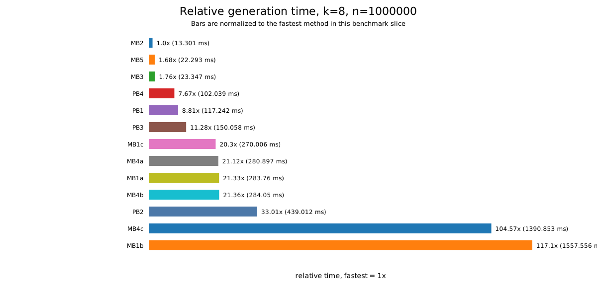
At k = 8 and n = 1_000_000, the retained table is:

The scaling plot shows the same run as a function of sequence length. These curves are most useful for relative behavior within one machine and Julia version, not as portable performance guarantees.

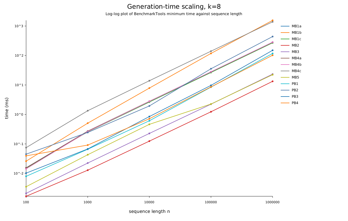
Benchmark labels include complexity-relevant settings such as k, d, stream count for FSS, copy-distance settings for DuplicationMutation, and FFT/rank-binning behavior for property-based methods. Interpret benchmark results as machine- and Julia-version-specific performance evidence, not as platform-independent speed guarantees.

The retained scaling run shows the expected separation between generator families: direct sequential methods are fastest, FFT/rank-binning methods scale well with sequence length, LGCM grows with alphabet size, and explicit history-based methods pay for their configured memory depth.